VLOOKUP function

Category: Lookup and reference functions

What does this function do?

Looking for a specific value in the first column of a table array and returns in the same row a value of another column of the table array.

Syntax:

VLOOKUP(lookup_value, table_array, col_index_num, [range_lookup])

• lookup_value (required): The value to search in the first column of the table or range. The lookup_value argument can be a value or a reference. If the value you supply for the lookup_value argument is smaller than the smallest value in the first column of the table_array argument, VLOOKUP returns the #N/A error value.

• table_array (required): The range of cells that contains the data. You can use a reference to a range (for example, A2:D8), or a range name. The values in the first column of table_array are the values searched by lookup_value. These values can be text, numbers, or logical values. Uppercase and lowercase text are equivalent.

• col_index_num (required): The column number in the table_array argument from which the matching value must be returned. A col_index_num argument of 1 returns the value in the first column in table_array; a col_index_num of 2 returns the value in the second column in table_array, and so on.

• range_lookup (optional): A logical value that specifies whether you want VLOOKUP to find an exact match or an approximate match. If range_lookup is either TRUE or is omitted, an exact or approximate match is returned. If an exact match is not found, the next largest value that is less than lookup_value is returned. If the range_lookup argument is FALSE, VLOOKUP will find only an exact match. If there are two or more values in the first column of table_array that match the lookup_value, the first value found is used. If an exact match is not found, the error value #N/A is returned.

Examples:

Imagine that there is a table that has all workers of a company, with their salaries, hours of work, and others. The table would look like this (imagine that the table is in the range A1: D6)

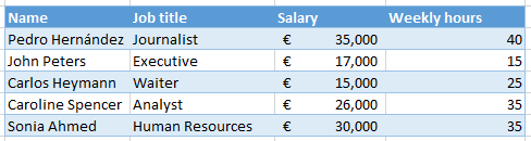
And you would like to know what the salary of Caroline Spencer is. This is where VLOOKUP function comes in handy.

= VLOOKUP ("Caroline Spencer", A1: D6, 3, FALSE)

The number 3 indicates that you want to return the salary that is located in the third column of the 'Employees' table.

False - means that we are looking for an exact match.

Suggestion:

1.Use almost always FALSE. It will be more accurate if what you want is to find the exact value.

2. Instead of "Caroline Spencer" is much better to introduce a cell reference. Imagine that the name you want to find is written in the cell R1 of your spreadsheet. It's better to write the formula as follows:
= VLOOKUP (R1, A1: D6, 3, FALSE)

3. Instead of a range like A1: D6, you should create a table for that that range and give it a name, eg 'Employees'
= VLOOKUP (R1, Employees, 3, FALSE)

4. Instead of True / False you can use 1/0. So the formula becomes:
= VLOOKUP (R1, Employees, 3, 0)