Dependent drop-down lists in Excel

In a recent entry I talked about how to insert drop-down lists in Excel. Today I would like to show you how to insert dependent drop-down lists. Basically what this means is to have 2 or more drop-down lists with the second one having as content a range that depends on the selection made in the first one. Look at the images below:

There is a drop-down list for a list of countries. Depending on the country chosen, the second drop-down list will display the list of cities from that country.

Conditional Formatting - Formula to highlight any day(s) of the week

Today we are looking at another example of using formulas in conditional formatting.

It is recommended to first read and understand the entrance Conditional Formatting - formulas for selecting cells

For this example we will use a normal list of days. In my case the list is in the range A1: A15.

Conditional Formatting - Formula to highlight alternate rows or columns

Here's an example of using conditional formatting formulas.

It is recommended to first read and understand the post Conditional Formatting - formulas for selecting cells

For this example we will use a normal table like this.

As can be clearly seen the table is for Moe's Tavern, and it shows a record of the daily sales.

1. Highlighting alternate rows

Conditional Formatting - formulas for selecting cells

An area where more flexibility is allowed in conditional formatting is the use of formulas for selecting which cells that must be formatted. In this section we will see examples of what kind of usages we can have with this option.

• Formula to highlight alternate rows or columns
• Formula to highlight specific day of the week
• Formula to highlight errors, omissions, repetitions
• Formula to highlight cells that contains a search value

-------------------------------------------------------------------------------------------------------------------------

But first let's see how a formula for conditional formatting is introduced.


1. First you have to go to Conditional Formatting> New Rule

Guide to Conditional Formatting in Excel

Conditional formatting in Excel is a very useful tool for analysing data and made it easy to give a special format to a group of cells based on value of another cell. Among the uses that can provide you is the power to apply a specific font or different fill colour to those cells that meet user-specified rules and thus facilitate their visual identification. Here I present a series of entries for better understanding of the tool.

1. Conditional Formatting - what it is and how to apply

2. Highlighting cells using conditional formatting

3. Formulas for selecting cells

• Formula to highlight alternate rows or columns

• Formula to highlight days of the week

• Formula to highlight errors, omissions, repetitions

• Formula to highlight cells that contains a search value

4. Conditional Formatting - Data Bars  (coming soon)

5. Conditional Formatting - Color Scales  (coming soon)

6. Conditional Formatting - Icon Sets  (coming soon)

7- Advanced techniques 1 (coming soon)

8- Advanced techniques 2 (coming soon)

Highlighting cells using conditional formatting

And what kind of effects can conditional formatting do?

1. Highlight cells rules

Operations that may occur;

• Greater than and/or equal to a value

• Less than and/or equal to a value

• Between 2 values

• Equal to a value

• Text containing ...

• A date occurring...

• Duplicates values

Conditional Formatting in Excel - what it is and how to apply

What is conditional formatting?

Conditional formatting in Excel is a very useful feature in the analysis of data as it empowers you to give a special format to a group of cells according to a condition(s). This format may be a different fill colour or a specific type of font for the cells that meet the established criteria so you can easily identify on the screen.

Although a special format could be given manually, conditional formatting creates an automatic formatting for cells that meet the specified condition, giving the user better visualisations.

Examples of conditional formatting

Highlighting maximum / minimum value of a series in a chart in Excel

Have you ever had a chart and wondered how you could highlight the maximum or minimum value of the series in that Excel chart.

We will discuss exactly that today.

Let's see how we can do it and create a chart like the one below:

Convert long NESTED IF formulas to a simple formula with the CHOOSE function

Anyone who has used Excel for a while will have found on more than one occasion long formulas that use the IF function inside another IF that in turn is inside another IF. This is normally called NESTED IF.

An easy example of NESTED IF would be:

= IF (B1 = 1, "Apple", IF (B1 = 2, "Orange", IF (B1 = 3 "Pera", "Grape")))


Obviously instead of the name of the fruits we could write a formula, or a cell.

= IF (B1 = 1, A1, IF (B1 = 2, A1-C1, IF (B1 = 3, A1 * D1, A1 ^ 2)))

How to build a Tornado chart in Excel

Hello! In this post I want to explain step by step how to build tornado chart in Excel. If you are a little confused about what a tornado chart is then let me show you visually. Basically a tornado chart looks like this (the typical graph of population distribution by age):

Drop-down lists in Excel

The drop-down list in Excel is a powerful tool that simplifies the process of choosing values ​​for the user. It is a technique widely used in which we can create lists that have the source data located on another sheet in Excel, which are hidden from the main sheet.

In this post we will look at two ways to create a drop-down list, first using data validation and then using the form control option.

1. Drop-down list with data validation

Guide to PivotTables in Excel

PivotTables are a very powerful tool to analyse data stored in Excel. In this tutorial we will see all the basics of PivotTables.

To enjoy the full tutorial is advisable to download the following file containing all the examples that are used.

PivotTables
------------------------------------------------------------------------------------------------------------------------


1. What are the PivotTables?

2. How to create a PivotTable

3. Formatting a PivotTable

4. Filtering PivotTables

5. Five cool tricks to PivotTables (coming soon)

6. Advanced Techniques for PivotTables (coming soon)

      1. Able to create monthly, quarterly and annual reports from daily data.
      2. Use the filter reports and generate multiple reports
      3. Slicers in PivotTables

Filtering PivotTables

Let's see how PivotTables are filtered

There are 2 possibilities to filter PivotTables:

1. Filter on a value of a variable that has been selected in the Filter field

In our previous example (I recommend reading this post), we had the following:

Formatting a PivotTable

And how do we format a PivotTable?

Let's suppose that we have the following PivotTable (I recommend you check this post):

Now we will format this report a bit.

What are PivotTables?

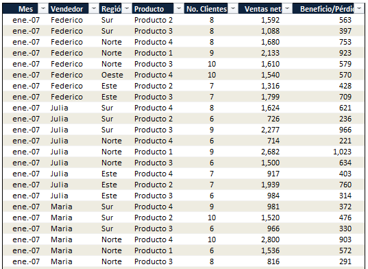
PivotTables in Excel are a powerful tool that helps us to conduct a thorough analysis of our data, making it quite easy for you to slice and dice, filter, sort and group information in the dynamic table according to our needs.

Basically they are a type of table that allow us to decide which variables appear as columns, as rows and as values ​​in the table and allow you to modify the structure quickly.

What are PivotTables for?

How to create a PivotTable

Let's see how to create a PivotTable

1. Imagine you have some sales data by salesperson, product and region. Make sure that the data has all column headers or table headers and that there are no blank rows .

2. Click any cell in the range of cells or table.