Highlighting cells using conditional formatting

And what kind of effects can conditional formatting do?

1. Highlight cells rules

Operations that may occur;

• Greater than and/or equal to a value

• Less than and/or equal to a value

• Between 2 values

• Equal to a value

• Text containing ...

• A date occurring...

• Duplicates values

Example:

Let's highlight cells that are greater than a value, for example 4, from the following list:

To highlight cells that are greater than 4, do the following:

• First select our range of cells

• Go to Conditional Formatting> Highlight cells rules > Greater than

• Introduce the value 4 to apply the conditional formatting. In this example the format will light red fill with dark red text, but that can be customised by the user.

• And the result is:

• To apply conditional formatting to cells that are less than a value, equal to value, text containing, you would need to do it in the same way, by simply selecting the desired option. To highlight cells between two values, you have to enter two values.

• The date option displays a list of options from where you can choose one. You will need date type data for this option to be applied.

• The last option will allow you to highlight duplicate values or unique values from a list of values. To achieve this, simply select the Duplicate Values option and then select Duplicate / Unique depending on what you intend to do, and identify what special format you want to apply.

2. Top/bottom Rules

The operations that can be done here are:

• The top 10 (or any other number) highest/lowest items

• Top 10% (or other percentage) of highest/lowest items

• Values above/below average

To do this, go to:

Conditional Formatting> Top/bottom Rules

• Select the data to apply conditional formatting

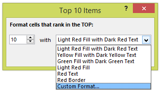
• Let's do the first choice, the top 10 items ... As you can see the number 10 can be changed to any number required and the type of format can also edited as there is an option called custom format.

• To apply conditional formatting for the bottom 10 items can be done in the same way by selecting Bottom 10 Items

• Now let's check the option for Top 10% of values. The rate and format can be changed in the same way we have just seen. This option will format the top 10% of the values, ie, if you have a list of 100 values, it will highlight the top 10% of the values based on value, which is obviously the 10 highest values.

• To do the Bottom 10% of the values would be done in a similar way by choosing the option Bottom 10%.

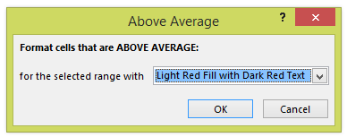
• Finally the option Above average does two things, calculate the average of the cells in the selected range and then apply conditional formatting to all those cells that have a value above the newly calculated average. Option Below Average select all cells that are smaller than average value.

To see more of conditional formatting click here.