How to create a PivotTable

Let's see how to create a PivotTable

1. Imagine you have some sales data by salesperson, product and region. Make sure that the data has all column headers or table headers and that there are no blank rows .

2. Click any cell in the range of cells or table.



3. Click the Menu Insert> PivotTable

4. Once you have clicked on PivotTable , it will show the dialog box Create PivotTable.

There you can adjust or set the table or range where you have stored your data and the destination where to place the PivotTable, which may be in the same sheet where your data is or in a different one, or even in a new book .

After selecting the table and location press OK and the PivotTable will be created.

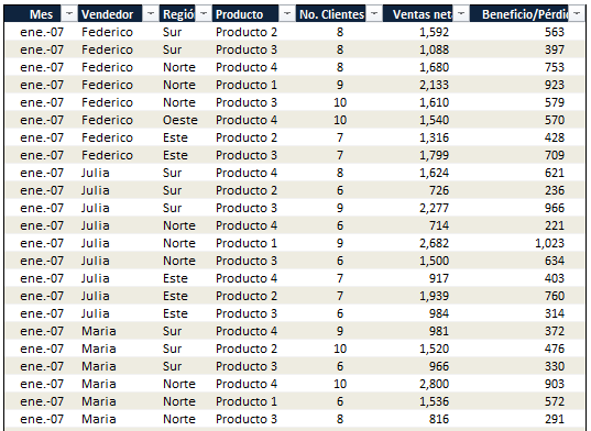
5. After adding the PivotTable, we have the following:

In Excel, the PivotTable is added on the left side of the book and the PivotTable fields on the right side. This PivotTable fields are divided into two sections, first a list of all fields among which we can choose and below an area where fields go either as column, row, value or filter .

To complete the PivotTable you must drag the fields to the corresponding area.

In my example, I will drag Salesperson to Columns, Region to Rows and Product to Filter. I will drag Net sales to value box.

The result would look like this:

And in such an easy way we created this PivotTable report sum of net sales by salesperson and region.